Conductors and Insulators
Elements of an Atom
Everything around us is made up of tiny particles called atoms. Each atom has a central core, the nucleus, surrounded by electrons in constant motion. The nucleus contains protons (positively charged) and neutrons (no charge). Electrons carry a negative charge (-). In a stable atom, the number of electrons equals the number of protons, resulting in a balanced charge.
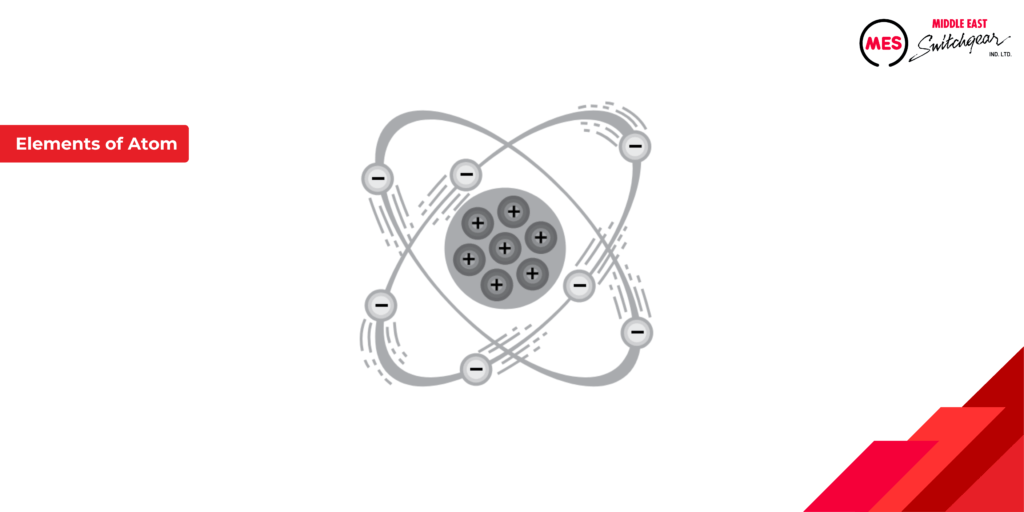
Table of Contents
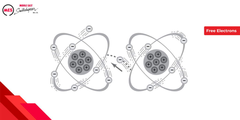
Free Electrons
Electrons occupy various energy levels around the nucleus. Electrons closer to the nucleus are more tightly bound. Electrons in the outermost shell can be dislodged by external forces like magnetic fields, friction, or chemical reactions. These dislodged electrons are called free electrons. A free electron leaving an atom creates a vacancy that another electron can fill.
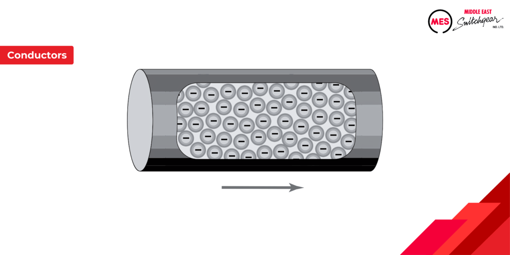
Conductors
Electrical Current
An electric current is produced when free electrons move from atom to atom in a material. Materials that permit many electrons to move freely are called conductors. Copper, silver, gold, aluminum, zinc, brass, and iron are considered good conductors. Of these materials, copper and aluminum are the ones most commonly used as conductors.
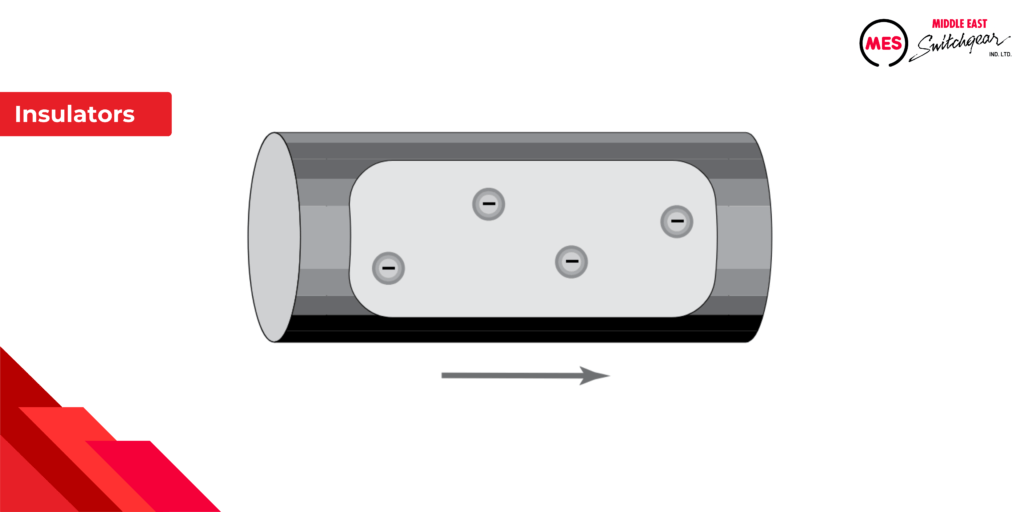
Insulators
Materials that impede the flow of free electrons are called insulators. Examples of good insulators include plastic, rubber, glass, mica, and ceramic.
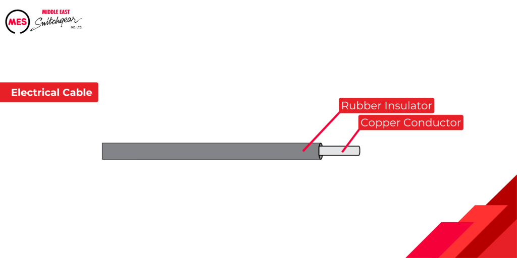
Electrical Cables
Electrical cables showcase the combined application of conductors and insulators. Electrons flow through a copper or aluminum conductor to power devices like radios, lamps, or motors. The insulator surrounding the conductor confines the electrons within the conductor.
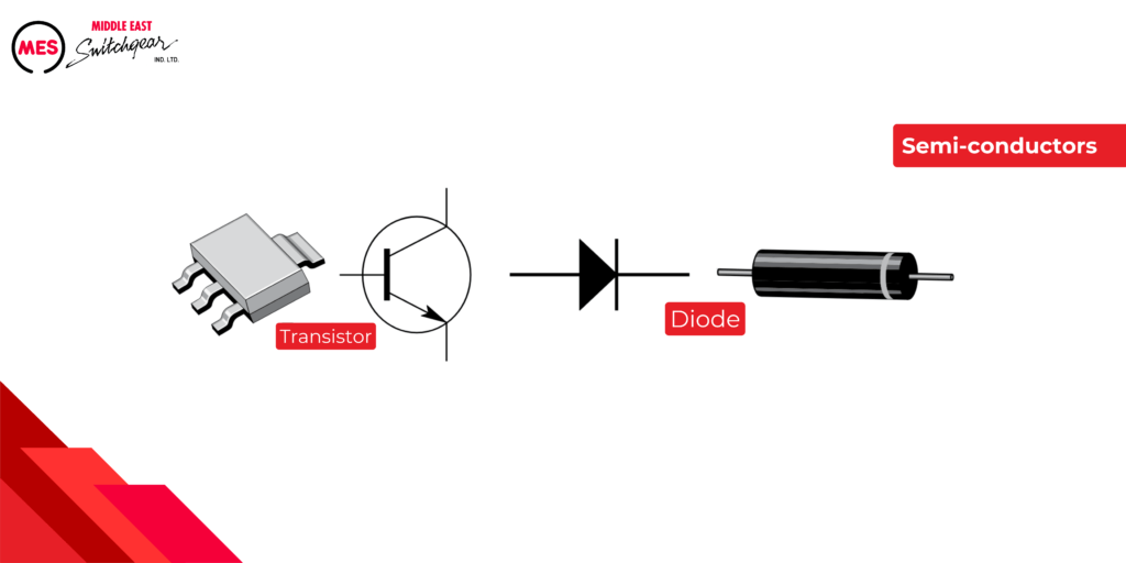
Semi-Conductors
Semiconductors, like silicon, are used to create devices with characteristics of both conductors and insulators. Certain semiconductors act like conductors when an external force is applied in a specific direction and like insulators when the force is applied in the opposite direction. This principle forms the basis for transistors, diodes, and other solid-state electronic devices.
Current, Voltage, and Resistance
Elements and Electrical Charges
All matter is composed of elements, each containing a single type of atom. Elements are identified by the number of protons and electrons in their atoms. For instance, a hydrogen atom has one proton and one electron, while an aluminum atom has 13 protons and 13 electrons. An atom with equal numbers of protons and electrons is electrically neutral.
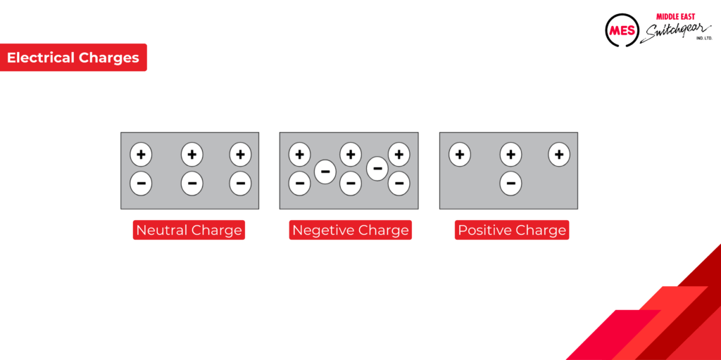
Electrical Charges
Electrons in an atom’s outer shell are susceptible to displacement by external forces. When an electron is dislodged, the atom becomes positively charged due to having more protons than electrons. Conversely, an atom or molecule can gain electrons, resulting in a negative charge. In essence, positive or negative charges arise from an imbalance of electrons, with the number of protons remaining constant.
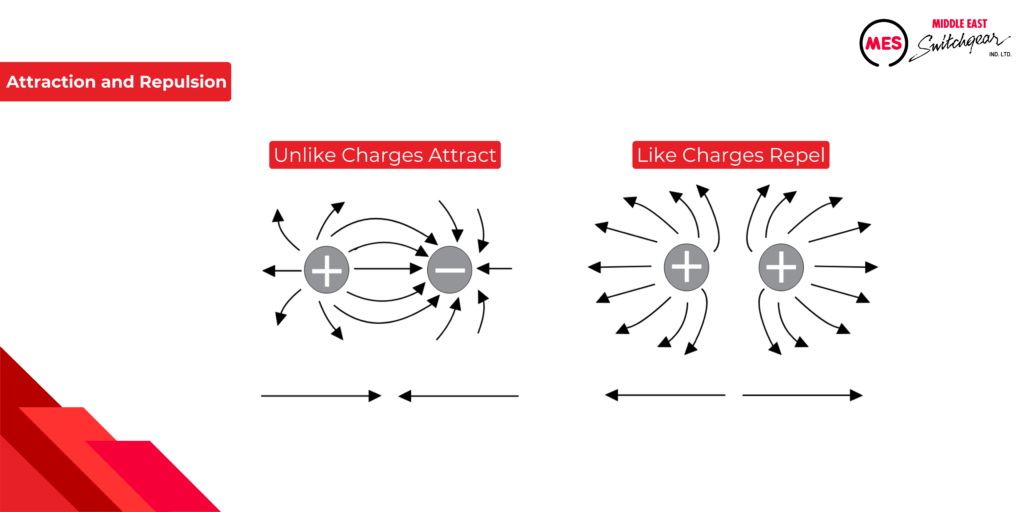
Attraction and Repulsion of Electric Charges
The familiar adage “opposites attract” holds true in the fascinating world of electric charges! These charges, either positive or negative, aren’t alone. They’re surrounded by invisible electric fields, acting like lines of force. Imagine these lines as invisible threads connecting the charges.
- Opposites Attract: When two objects have opposite charges (positive and negative), their electric field lines connect them, pulling the objects together. Think of it as opposite sides of a magnet, drawn to each other.
- Likes Repel: But if both objects share the same charge (both positive or both negative), their electric field lines push against each other, causing the objects to repel and move apart. Imagine two similar magnetic poles trying to push each other away.
By understanding these interactions between electric charges and their invisible fields, we unlock the fundamental principles of electricity that power our everyday lives!
Current
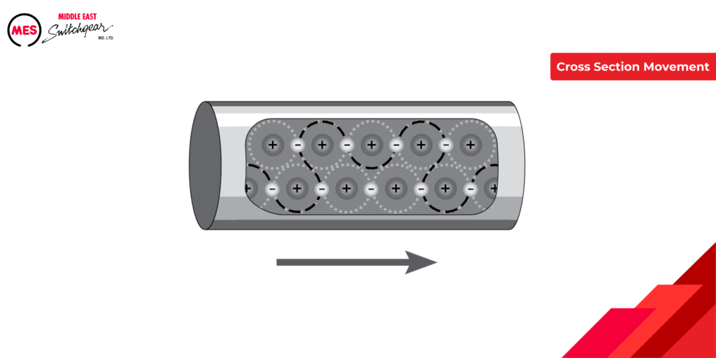
In the field of electrical engineering, current (denoted by the symbol I) represents the directed movement of free electrons through a conductor. These free electrons, freed from their atomic nuclei, collectively move from one atom to the next in a unified direction. The current’s magnitude is directly proportional to the number of electrons passing through a specific cross-sectional area of the conductor per unit time (usually one second).
In simple terms, current indicates the flow rate of these mobile charges. A larger quantity of electrons moving through a conductor in a given period results in a higher current value. This fundamental concept forms the basis of electrical circuits and their ability to supply power to various electronic devices.
It’s important to remember that atoms are incredibly small. In a copper conductor, it takes about 10^24 atoms to fill one cubic centimeter. Representing even a small value of current as electrons would result in an extremely large number. That’s why current is measured in amperes, often shortened to amps, with the symbol A. One amp of current means that about 6.24 x 10^18 electrons move through a cross-section of the conductor in one second. While these numbers are provided for informational purposes, it’s crucial to understand the concept of current flow. Electrical units often use metric prefixes to represent powers of ten, as there can be wide variations in the magnitude of electrical quantities. The following chart illustrates how three of these prefixes are used to represent large and small values of current.
UNIT
SYMBOL
Equivalent Measure
kiloampere
kA
1 kA = 1000 A
milliampere
mA
1 mA = 0.001 A
microampere
µA
1 µA = 0.000001 A
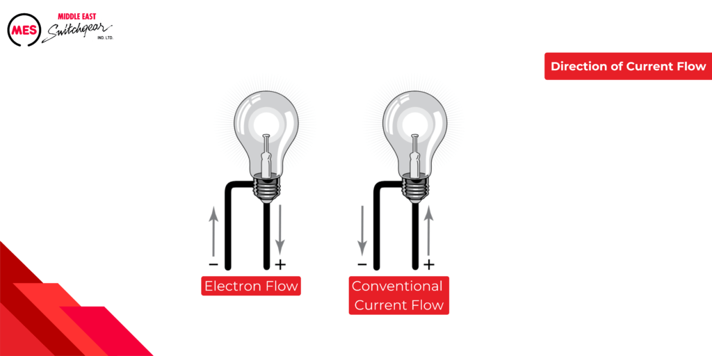
Direction of Current Flow
Within the field of electrical engineering, the concept of current flow can generate some discussion. Traditionally, there exist two primary perspectives:
Conventional Current Flow: This established approach simplifies the concept by disregarding the actual movement of electrons and instead postulates that current flows from positive to negative terminals in a circuit.
Electron Flow: This approach aligns more directly with the physical phenomenon, acknowledging the movement of free electrons within a conductor. These negatively charged particles migrate from a region of higher concentration (negative terminal) to a region of lower concentration (positive terminal), establishing the current.
To maintain scientific accuracy and reflect the underlying physics, this course utilizes the electron flow concept. This signifies that a current is established by the directed movement of negatively charged electrons.
Voltage
In the realm of electrical engineering, voltage, also known as potential difference or electromotive force (EMF), signifies the energy per unit charge that compels the flow of electricity through a conductor. This essential concept is denoted by the symbol E or V, and its unit of measurement is the volt (V).
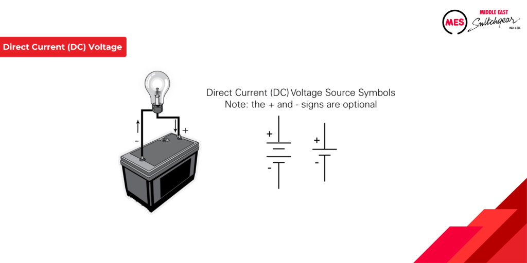
Voltage can be generated through various mechanisms. Batteries, for instance, rely on an electrochemical process, while car alternators and power plant generators leverage the principle of magnetic induction. A defining characteristic of all voltage sources is the presence of an imbalanced electron distribution, with an excess at one terminal (typically negative) and a deficit at the other (typically positive). This disparity creates a potential difference between the terminals, driving the movement of electrons and establishing an electric current.
In the case of a direct current (DC) voltage source, the polarity of the terminals remains constant. Consequently, the resulting current consistently flows in a single direction within the circuit.
The following chart shows how selected metric unit prefixes are used to represent large and small values of voltage.
Unit
Symbol
Equivalent Measure
kilovolt
kV
1 kV = 1000 V
millivolt
mV
1 mV = 0.001 V
microvolt
µV
1 µV = 0.000001 V
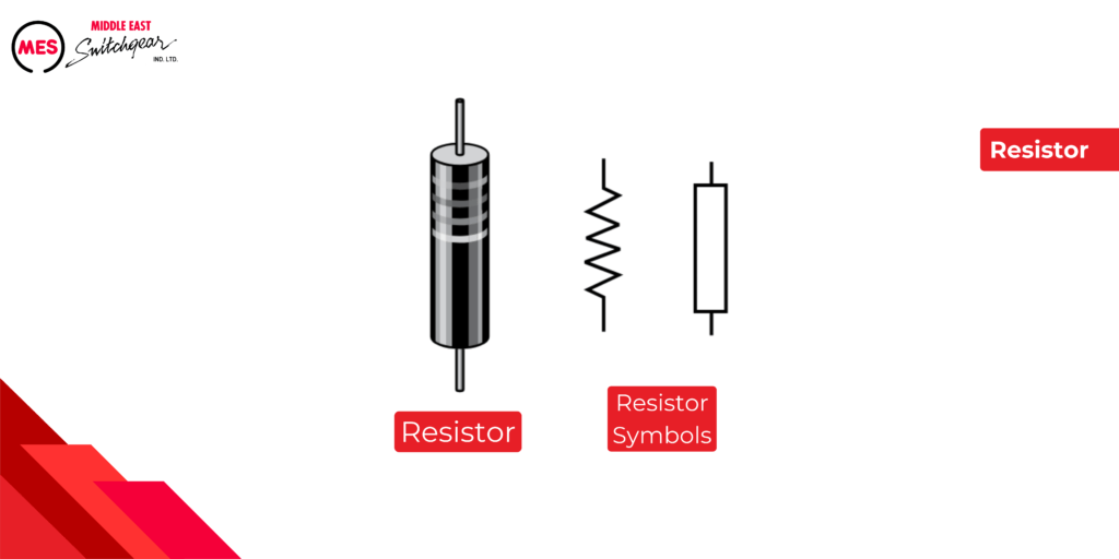
Resistance
Electrical circuits involve a fundamental concept called resistance, denoted by the symbol R. Measured in ohms (Ω), resistance signifies the inherent opposition a material presents to the flow of electric current. In essence, it acts as a counterforce, hindering the movement of charged particles.
The degree of resistance is influenced by several key factors:
- Material Composition: Different materials possess varying inherent resistance properties. For example, conductors like copper exhibit low resistance, while insulators like rubber offer very high resistance.
- Length: Generally, the longer a conductor, the greater its resistance. Imagine a longer path for electrons to navigate.
- Cross-Sectional Area: A conductor’s resistance is inversely proportional to its cross-sectional area. Think of a wider pipe offering less resistance to water flow compared to a narrow one.
- Temperature: Resistance often increases with rising temperature in conductors.
Understanding these factors and their impact on resistance is crucial for designing efficient electrical circuits.
In addition to resistors, all other circuit components and the conductors that connect components to form a circuit also have resistance.
The basic unit for resistance is 1 ohm; however, resistance is often expressed in multiples of the larger units shown in the following table.
Unit
Symbol
Equivalent Measure
megaohm
MΩ
1 MΩ = 1,000,000 Ω
kilohm
kΩ
1 kΩ = 1000 Ω
Ohm's Law
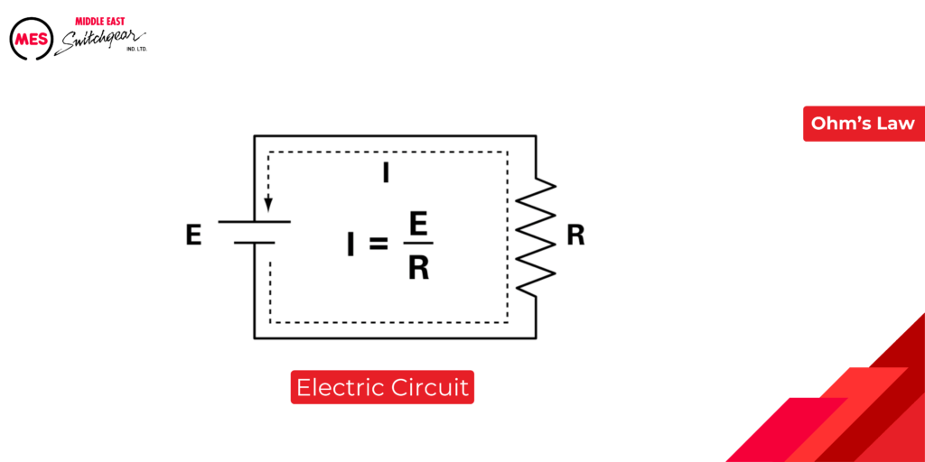
Electric Circuit
A fundamental electrical circuit comprises three key elements:
- Voltage Source: This component, like a battery or generator, provides the driving force (electromotive force or EMF) that propels electrons through the circuit.
- Load: This represents the element within the circuit that utilizes the electrical energy. Examples include lamps, motors, or electronic devices.
- Conductors: These components, typically wires made of low-resistance materials like copper, serve as pathways for the flow of electrons between the voltage source and the load.
Ohm’s Law, a cornerstone of electrical engineering, governs the relationship between these elements:
- Current (I): The rate of electron flow within the circuit, measured in amperes (A).
- Voltage (V): The potential difference or electromotive force provided by the voltage source, measured in volts (V).
- Resistance (R): The opposition to current flow inherent in the circuit, measured in ohms (Ω).
Ohm’s Law states that current is directly proportional to voltage and inversely proportional to resistance. Mathematically, this can be expressed as I = V / R. Understanding this relationship is essential for analyzing and designing electrical circuits effectively.
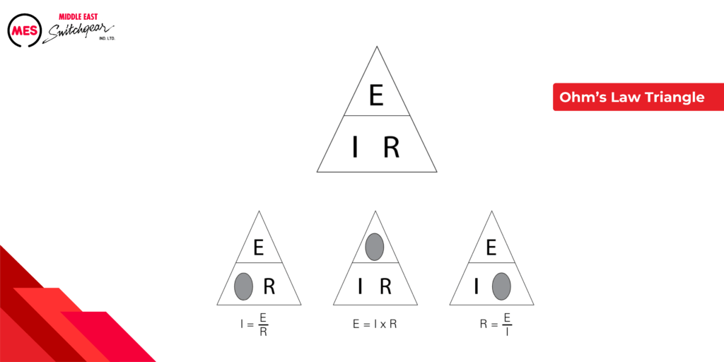
Ohm's Law Triangle
Ohm’s Law provides a powerful tool for analyzing electrical circuits. However, for those new to the field, remembering the specific formulas (I = V/R, V = IR, R = V/I) can be challenging.
While some techniques, like the mnemonic triangle you may have encountered, can aid in memorization, a more practical approach might be beneficial. By focusing on the relationship between the three variables, you can readily derive the correct formula:
- Current (I) is directly proportional to Voltage (V) and inversely proportional to Resistance (R).
Based on this understanding, you can rearrange the variables to solve for the desired quantity:
- To find Current (I): I = V / R
- To find Voltage (V): V = I * R
- To find Resistance (R): R = V / I
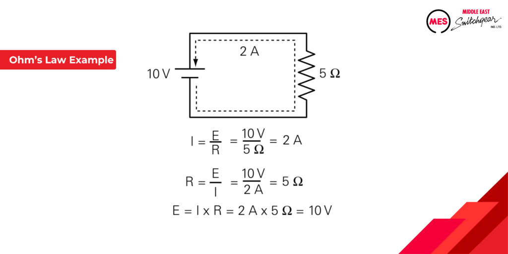
Ohm's Law Example
As the following simple example shows, if any two values are known, you can determine the other value using Ohm’s law
Using a similar circuit, but with a current of 200 mA and a resistance of 10 W.To solve for voltage, cover the E in the triangle and use the resulting equation.
E = I x R E = 0.2 A x 10 Ω = 2 V
Remember to use the correct decimal equivalent when dealing with numbers that are preceded with milli (m), micro (m), kilo (k) or mega (M). In this example, current was converted to 0.2 A, because 200 mA is 200 x 10-3 A, which is equal to 0.2 A.
DC Circuits
Series Circuits
In electrical engineering, a series circuit represents a configuration where multiple components are connected end-to-end. This arrangement creates a single, unified pathway for current to traverse through the circuit. Imagine a single-lane road – electrons can only flow in one direction through the connected components.
Consider the following illustration: five resistors are connected in series. The current has no choice but to flow from the negative terminal of the voltage source, passing consecutively through all five resistors, before returning to the positive terminal. This single current path is a defining characteristic of series circuits.
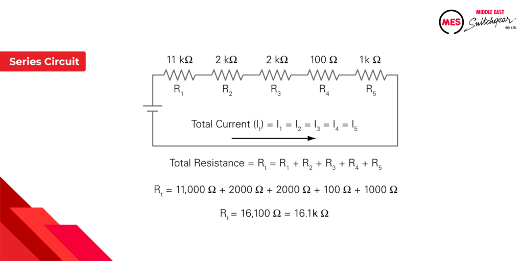
Key Characteristics of Series Circuits:
- Total Resistance (Rt): The overall resistance (measured in ohms, Ω) in a series circuit is simply the sum of the individual resistor values. However, it’s crucial to ensure all resistance values are in the same unit before summation. Metric prefixes like kilo (kΩ) or mega (MΩ) are often used, so conversions might be necessary.
- Current (I): Ohm’s Law (I = V/R) governs the current flow in a series circuit. Here, V represents the source voltage and R represents the total resistance (sum of individual resistors). The calculated current value remains constant throughout the entire series circuit.
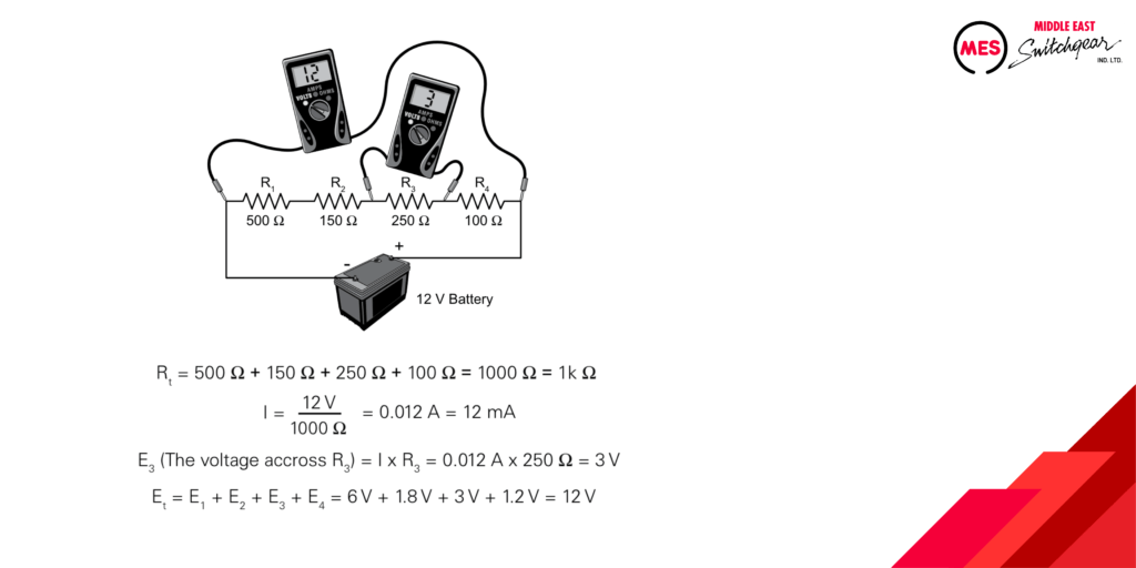
- Voltage Drops (Vd): The voltage across each resistor in a series circuit can also be determined using Ohm’s Law. This voltage drop (Vd) is specific to each resistor and depends on its individual resistance value and the overall current.
- Source Voltage and Voltage Drops: Interestingly, the sum of the voltage drops across all resistors in a series circuit is always equal to the total voltage supplied by the source. This principle reflects the conservation of energy within the circuit.
The following illustration shows two voltmeters, one measuring total voltage and one measuring the voltage across R3.
Parallel Circuits
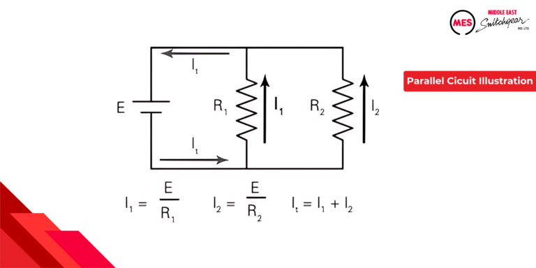
Parallel circuits represent another essential configuration in electrical engineering. Unlike series circuits, they offer multiple pathways for current to flow simultaneously. Imagine a multi-lane highway – electrons have the option to travel through various branches depending on the resistance offered by each path.
Consider the following illustration: a simple parallel circuit with two resistors connected side-by-side. This arrangement creates two distinct current paths:
- Path 1: Current flows from the negative terminal of the battery, through resistor R1, and returns to the positive terminal.
- Path 2: Current simultaneously flows from the negative terminal of the battery, through resistor R2, and returns to the positive terminal.
Determining Current in a Parallel Circuit:
The current flowing through each individual resistor in a parallel circuit can be calculated using Ohm’s Law (I = V/R), where:
- I represents the current in amperes (A)
- V represents the total source voltage in volts (V)
- R represents the resistance of the specific resistor in ohms (Ω)
The total resistance for a parallel circuit with any number of resistors can be calculated using the formula shown in the following illustration.
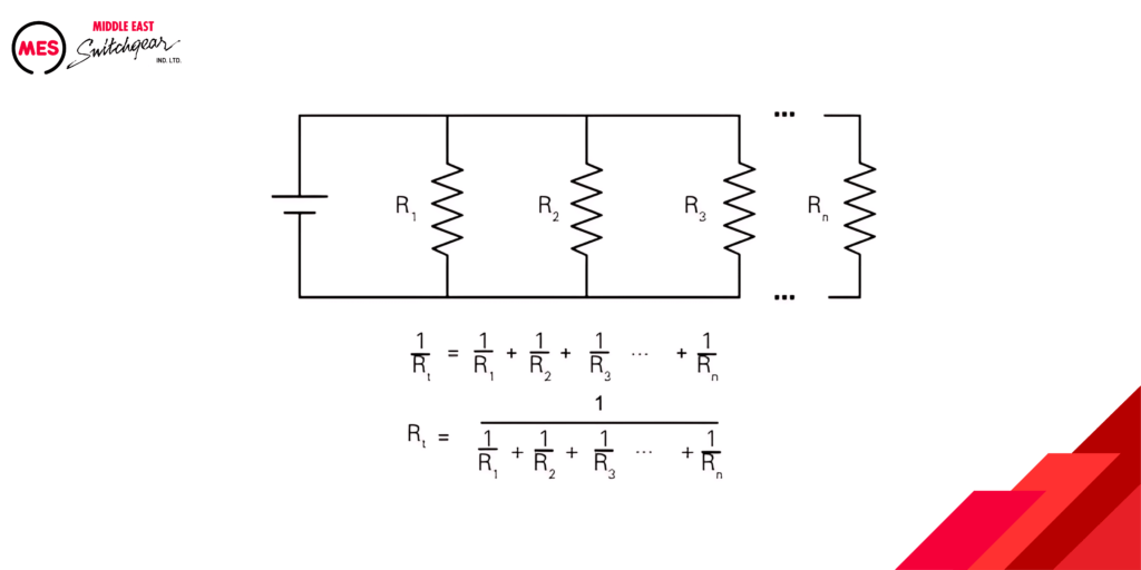
In the unique example where all resistors have the same resistance, the total resistance is equal to the resistance of one resistor divided by the number of resistors. The following example shows a total resistance calculation for a circuit with three parallel resistors.
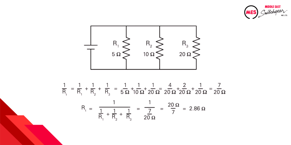
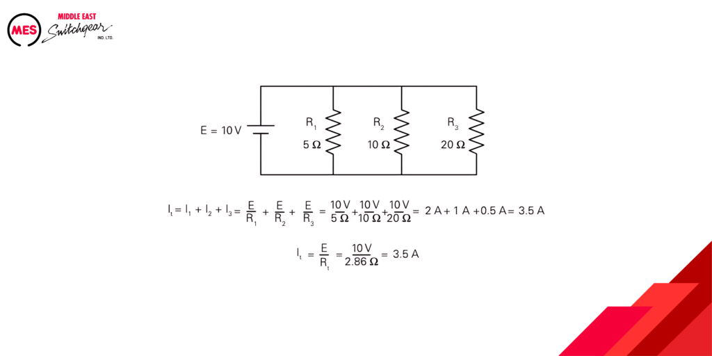
Current in each of the branches of a parallel circuit can be calculated by dividing the circuit voltage, which is the same for all branches, by the resistance of the branch.The total circuit current can be calculated by adding the current for all branches or by dividing the circuit voltage by the total resistance.
Series-Parallel Circuit
Electrical circuits can become more intricate by combining series and parallel connections. These configurations are known as series-parallel circuits or compound circuits. They require at least three components and offer more flexibility in designing circuits with specific electrical characteristics.
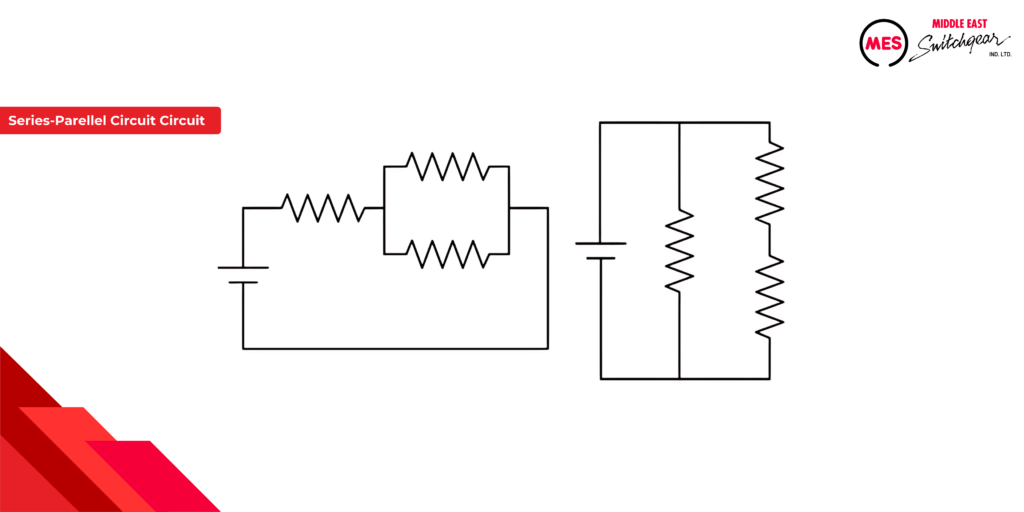
The provided illustration showcases two basic series-parallel circuit examples:
- Left Circuit: This configuration features two resistors connected in parallel, with the combined pair then connected in series with another individual resistor.
- Right Circuit: This circuit involves two resistors connected in series, with the combined series combination then connected in parallel with another individual resistor.
By understanding how current flows through these combined configurations, engineers can design circuits for various applications.
Series-parallel circuits, also known as compound circuits, represent an extension of the basic series and parallel configurations. They involve a combination of these structures to achieve more complex functionalities within a circuit. While these circuits can appear intricate, a systematic approach using the previously discussed circuit analysis principles can simplify the process.
Key Points for Series-Parallel Circuit Analysis:
- Fundamental Building Blocks: Series-parallel circuits require at least three components and are built upon a foundation of understanding both series and parallel configurations.
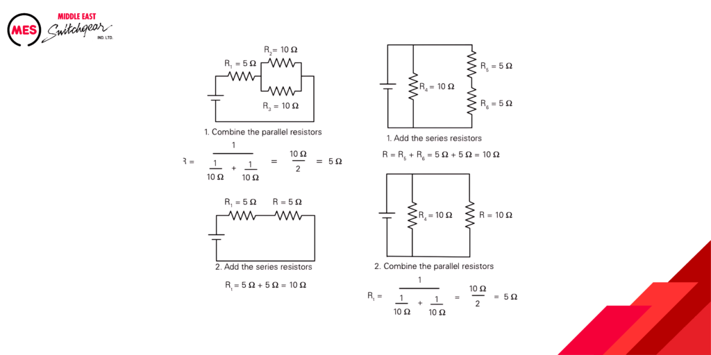
- Step-by-Step Analysis: By systematically breaking down the circuit into smaller, recognizable series or parallel combinations, the total resistance and ultimately other circuit characteristics can be determined. The provided illustration showcases how this step-by-step approach can be applied to two basic series-parallel circuits.
- Scalability of the Method: The same analytical approach can be applied to even more complex series-parallel circuits. While the number of steps might increase, each step remains relatively straightforward.
- Leveraging Ohm’s Law: Once the total resistance of the circuit is established, Ohm’s Law (I = V/R) can be utilized to determine current throughout the circuit. By applying Ohm’s Law to individual components, voltage drops across various elements can also be calculated.
By mastering these analysis techniques, engineers can effectively design and analyze series-parallel circuits for various electrical applications.
The following illustration shows how total resistance can be determined for two series-parallel circuits in two easy steps for each circuit. More complex circuits require more steps, but each step is relatively simple.
Power in a DC Circuit
The concept of power transcends various scientific disciplines, including electricity. In essence, whenever a force acts upon an object, causing it to move, work is done. In the context of electrical circuits, power signifies the rate at which electrical work is performed.
Voltage as the Driving Force:
Imagine voltage as a force pushing electrons through a conductor. This movement of electrons constitutes the “motion” associated with electrical work.
Power: The Rate of Work Done:
Power, denoted by the symbol P and measured in watts (W), reflects the rate at which this electrical work is accomplished. In a direct current (DC) circuit, one watt signifies the rate of work done when one volt (V) causes a current of one ampere (A) to flow.
Deriving Power Formulas:
The fundamental formula for electrical power in a DC circuit is P = VI (power equals voltage multiplied by current). This equation serves as the foundation for deriving other power-related formulas, particularly when dealing with alternating current (AC) circuits, which you’ll explore later. Ohm’s Law, a cornerstone of electrical analysis, plays a crucial role in these derivations.
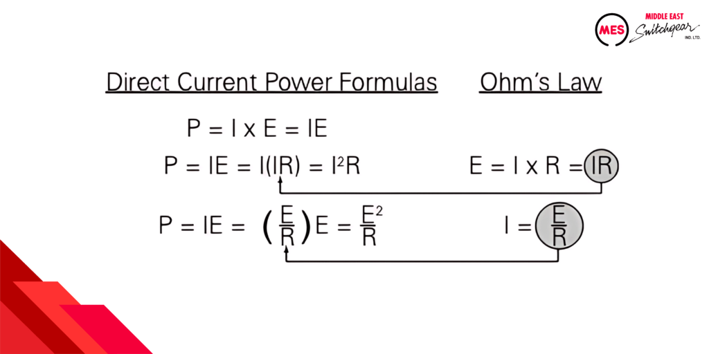
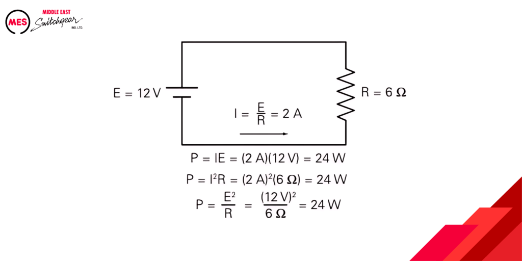
The following example shows how power can be calculated using any of the power formulas.
Magnetism
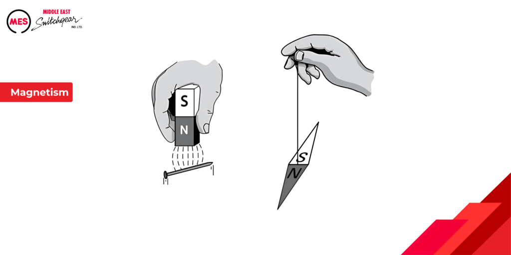
The realms of magnetism and electricity exhibit a fascinating interdependence. Not only are they fundamentally linked, but they can also be used to generate each other. While permanent magnets, often visualized as horseshoe or bar magnets, come in various shapes, they share two defining characteristics:
- Attraction to Iron: Permanent magnets inherently attract ferrous materials like iron.
- North-South Orientation: When free to move, a magnet aligns itself in a north-south direction, as exemplified by a compass needle.
Beyond Permanent Magnets:
It’s important to note that permanent magnets are just one facet of magnetism. This course will delve deeper into the fascinating interplay between magnetism and electricity, exploring concepts like:
- Electromagnets: These temporary magnets utilize electric current to generate a magnetic field, demonstrating the ability to create magnetism through electricity.
- Electromagnetic Induction: This phenomenon describes the generation of electric current through a conductor by a changing magnetic field. It highlights the reciprocal relationship where magnetism can induce electricity.
Understanding this interconnectedness is fundamental to various electrical applications, from motors and generators to transformers and inductors.
Magnetic Lines of Flux
Magnets possess a fascinating property known as polarity. Every magnet exhibits two distinct poles: a north pole and a south pole. These poles cannot exist independently – a magnet always has both.
Magnetic Fields: The Lines of Force
While invisible to the naked eye, magnets exert their influence through a surrounding magnetic field. Imagine these fields as lines of force emanating from the north pole and terminating at the south pole. These lines, though intangible, have a demonstrable effect.
Visualizing the Magnetic Field:
A simple experiment can reveal the presence of the magnetic field. Place a sheet of paper over a magnet and sprinkle iron filings on top. The iron filings, susceptible to the magnetic force, will align themselves along the invisible lines of flux, creating a visual representation of the magnetic field. This alignment demonstrates the attractive forces between the north pole of the magnet and the induced south poles in the iron filings, as well as the repulsive forces between the south pole of the magnet and the induced north poles in the filings.
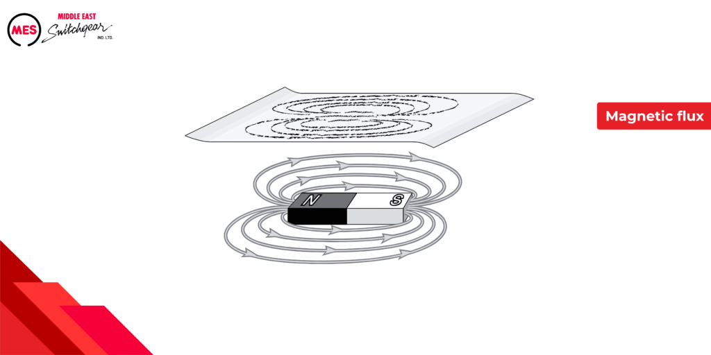
The density of these lines of flux is greatest inside the magnet and where the lines of flux enter and leave the magnet. The greater the density of the lines of flux, the stronger the magnetic field.
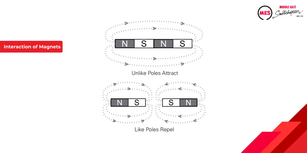
Interaction between Magnets
The interplay between magnets is governed by their surrounding magnetic fields, regions of invisible force. When two magnets are brought close together, their magnetic fields interact, leading to distinct behaviors:
- Attraction: When opposite poles (north and south) face each other, the magnetic force between them is attractive. Imagine the lines of flux from the north pole of one magnet converging with the lines of flux entering the south pole of the other, creating a pulling effect.
- Repulsion: Conversely, when like poles (north-south or south-south) are brought together, the magnetic force becomes repulsive. In this scenario, the lines of flux from similar poles try to push away from each other, resulting in a repelling force.
Understanding Magnetic Force:
This attractive or repulsive force arises from the interaction between the moving charged particles within each magnet. These interactions exert a force on the overall structure of the magnets, leading to the observed attraction or repulsion.
Electromagnetism
The electromagnetism centers around the concept of the electromagnetic field. This field arises from, and is intricately linked to, the flow of electric current in a conductor. In essence, every electric current generates a surrounding magnetic field.
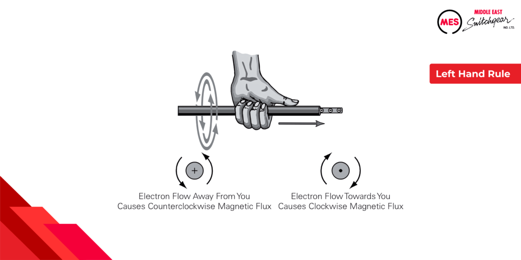
The Left-Hand Rule:
Understanding the relationship between current direction and the resulting magnetic field is crucial. Here’s where the left-hand rule for conductors comes into play. This rule provides a simple yet effective way to visualize the magnetic field generated by a current-carrying conductor:
- Grasp the Conductor: Imagine holding the current-carrying conductor in your left hand.
- Thumb Follows Electrons: Point your thumb in the direction of conventional current flow (which is opposite to the actual flow of electrons).
- Fingers Wrap Around the Field: Curl your fingers around the conductor. The direction your fingers encircle the conductor signifies the direction of the magnetic lines of flux associated with the current.
By following these steps, you can readily determine the magnetic field generated by a current-carrying conductor, even though the field itself is invisible.
Electromagnets offer a prime example of the captivating interplay between electricity and magnetism. These temporary magnets are essentially coils of wire that, when carrying an electric current, generate a magnetic field.
From Loops to Magnetic Fields:
Imagine each loop of wire within the coil acting like a tiny magnet, with its own magnetic field. The beauty of an electromagnet lies in how these individual fields combine. As the loops are stacked together in the coil, their magnetic fields add up, creating a significantly stronger overall magnetic field.
Factors Influencing Magnetic Strength:
The strength of an electromagnet’s magnetic field can be strategically manipulated through several key factors:
- Number of Turns: Increasing the number of loops or turns within the coil directly strengthens the resulting magnetic field.
- Current Flow: A higher current flowing through the coil translates to a more robust magnetic field.
- Core Material: Winding the coil around a core made of soft iron, a material that conducts magnetic flux more efficiently than air, significantly intensifies the magnetic field. Soft iron becomes magnetized in the presence of the current but readily loses its magnetism when the current ceases.
Widespread Applications of Electromagnets:
Electromagnets find application in a vast array of electrical devices due to their controllable magnetic fields. From the essential role they play in motors and generators to their functionality in circuit breakers, contactors, relays, and motor starters, electromagnets are a cornerstone of modern technology.
Alternating Current
The supply of current for electrical devices may come from a direct current (DC) source or an alternating current (AC) source. In a direct current circuit, electrons flow continuously in one direction from the source of power through a conductor to a load and back to the source of power. Voltage polarity for a direct current source remains constant. DC power sources include batteries and DC generators.
By contrast, an AC generator makes electrons flow first in one direction then in another. In fact, an AC generator reverses its terminal polarities many times a second, causing current to change direction with each reversal.
AC Sine Wave
In the realm of alternating current (AC) circuits, voltage and current values fluctuate continuously. To effectively analyze and understand these variations, we rely on a graphical representation known as the sine wave.
The Versatile Sine Wave:
The beauty of the sine wave lies in its ability to depict both AC voltage and current. It serves as a universal graphical language for visualizing these dynamic electrical quantities.
Decoding the Axes:
The sine wave rests upon a two-axis system:
- Vertical Axis (Y-axis): This axis represents the magnitude and direction (positive or negative) of either AC voltage or current. The peak value of the wave corresponds to the maximum magnitude of the quantity being represented.
- Horizontal Axis (X-axis): Time is the domain of the horizontal axis. As we move along this axis from left to right, we track the variations in voltage or current over time.
Understanding the Shape:
The characteristic shape of the sine wave resembles a smooth, continuous curve that oscillates above and below a central zero line. This oscillation reflects the ever-changing nature of AC voltage and current.
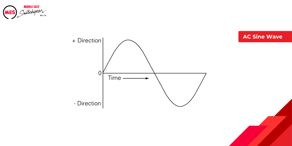
The sine wave is a powerful tool for understanding AC circuits. Its position above or below the time axis reflects current direction (positive or negative). Each complete wave cycle (360°) represents one cycle of AC voltage or current variation. We’ll delve into AC frequency next, which tells us how many cycles occur per second.
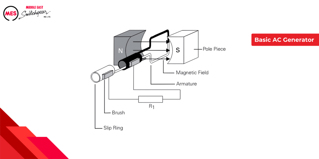
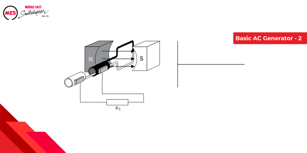
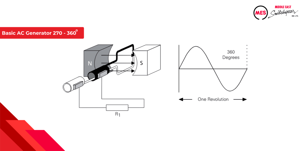
Basic AC Generator
At its core, a simple generator has a rotating loop of wire (armature) spinning within a magnetic field. This movement induces a voltage in the wire, causing current to flow. Here’s a breakdown of the key parts:
- Magnetic Field: Provides the invisible force that interacts with the moving wire.
- Armature: A single loop of wire in this example, but typically consists of multiple coils for increased efficiency.
- Slip Rings: Rotating contacts that connect the armature to the external circuit.
- Brushes: Conduct electricity from the rotating slip rings to the load.
- Resistive Load: The element, like a light bulb, that utilizes the generated current.
As the armature spins, the changing magnetic field induces a voltage in the loop. The slip rings and brushes transfer this generated current to the load, completing the circuit and powering the device.
An armature rotates through the magnetic field. At an initial position of zero degrees, the armature conductors are moving parallel to the magnetic field and not cutting through any magnetic lines of flux. No voltage is induced.
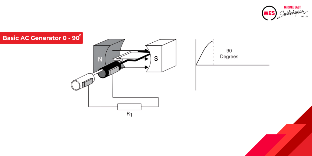
Generator Operationn from Zero to 90 Degrees
At its core, a simple generator has a rotating loop of wire (armature) spinning within a magnetic field. This movement induces a voltage in the wire, causing current to flow. Here’s a breakdown of the key parts:
- Magnetic Field: Provides the invisible force that interacts with the moving wire.
- Armature: A single loop of wire in this example, but typically consists of multiple coils for increased efficiency.
- Slip Rings: Rotating contacts that connect the armature to the external circuit.
- Brushes: Conduct electricity from the rotating slip rings to the load.
- Resistive Load: The element, like a light bulb, that utilizes the generated current.
As the armature spins, the changing magnetic field induces a voltage in the loop. The slip rings and brushes transfer this generated current to the load, completing the circuit and powering the device.
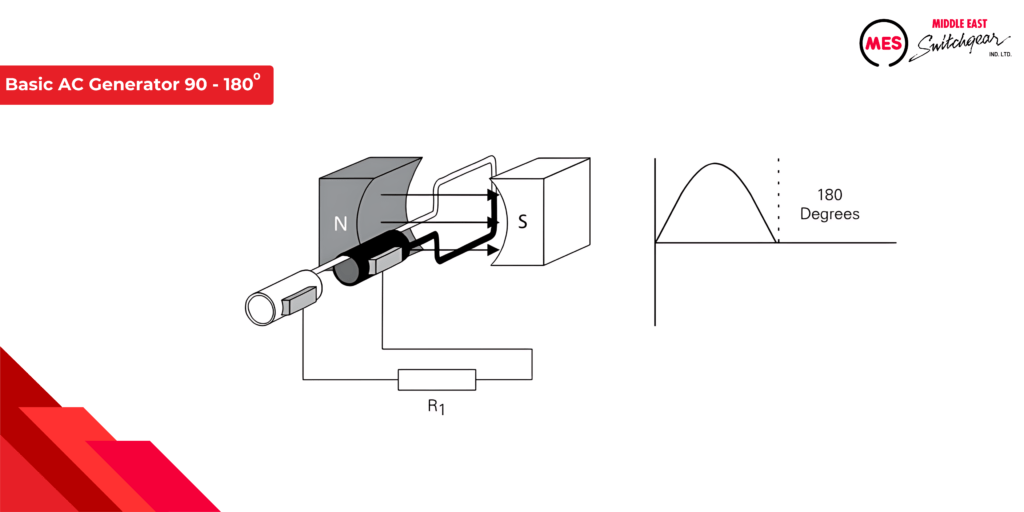
Generator Operation from 90 to 180 degrees
The armature continues to rotate from 90 to 180 degrees, cutting fewer lines of flux.The induced voltage decreases from a maximum positive value to zero.
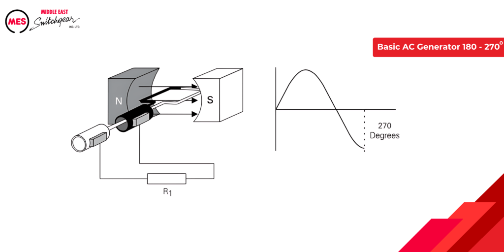
Generator Operation from 180 to 270 degrees
As the armature rotates from 180 to 270 degrees, the conductors cut through more magnetic flux lines in the opposite direction. This induces a voltage that increases negatively, peaking at 270 degrees.
Generator Operation from 270 to 360 degrees
As the armature progresses from 270 to 360 degrees of rotation, the induced voltage diminishes from its maximum negative value to zero, marking the culmination of one cycle. This continuous rotation at a consistent speed ensures the repetition of the cycle as long as the armature remains in motion. Understanding this cyclic process is vital for optimizing the performance of electric motors and ensuring their sustained efficiency across various operational scenarios.
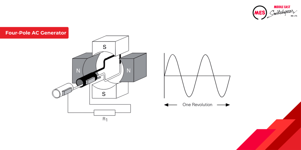
Four-Pole AC Generator
AC Generator Poles & Frequency: More Poles, Higher Frequency
The number of poles in an AC generator directly impacts the frequency (cycles per second) of the electricity it produces. More poles = higher frequency at the same rotation speed (think cycles per revolution). This allows engineers to design generators for various applications by adjusting poles and speed.
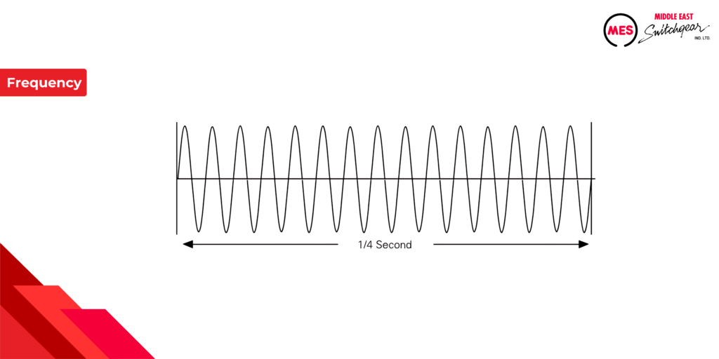
Frequency
The passage you provided accurately explains the connection between AC generator poles, rotation speed, and frequency. Here’s a concise breakdown:
- AC generator frequency is the number of voltage cycles produced per second, measured in Hertz (Hz).
- Poles and Frequency: More poles in the generator lead to higher frequency at a constant rotation speed (e.g., a 2-pole generator at 60 rotations/second produces 60 Hz).
- Common Frequencies: Power grids use either 60 Hz (US) or 50 Hz (Europe) for electricity distribution.
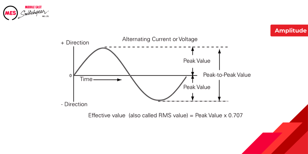
Amplitude
We’ve learned that AC voltage and current follow a sine wave pattern, with both frequency (cycles per second) and amplitude (strength of variation). Here’s how we measure amplitude:
- Peak Value: Highest point reached by the wave (positive or negative).
- Peak-to-Peak Value: Total distance between the wave’s peak and trough (twice the peak value).
- Effective (RMS) Value: The most practical measure, representing AC’s heating effect equivalent to DC. This is what most AC meters display and is roughly 0.707 times the peak value.
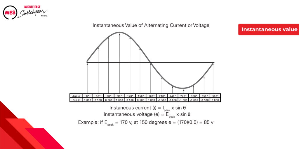
Every point on a sine wave has an “instantaneous value,” representing the voltage or current at that specific moment. This value is related to the sine function.
While the illustration might only show values at 30-degree intervals, each point has a unique value. We can calculate it using the formula:
- Instantaneous value = Peak value x sin(θ)
Here, θ (theta) represents the angle in degrees along the wave, and sin(θ) is its sine value obtained from trigonometric tables.
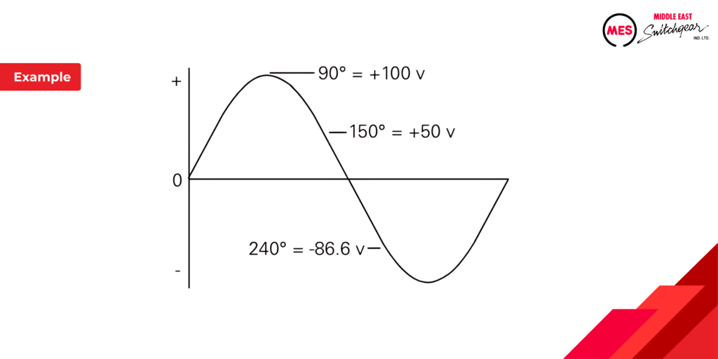
The following example illustrates instantaneous values at 90, 150, and 240 degrees for a peak voltage of 100 volts. By substituting the sine at the instantaneous angle value, the instantaneous voltage can be calculated.
Inductance and Capacitance
Inductance
Circuits aren’t just about resistance. Inductance is another property that affects current flow. Unlike resistance, which simply opposes the current itself, inductance opposes changes in the current. It’s denoted by L and measured in henrys (H), but smaller units like millihenrys (mH) are common.
How it Works:
- Current creates a magnetic field around the conductor.
- Any change in current (like in AC circuits) causes this field to change as well.
- This changing magnetic field induces a voltage in the conductor itself, opposing the original current change. This is called counter-electromotive force (counter EMF).
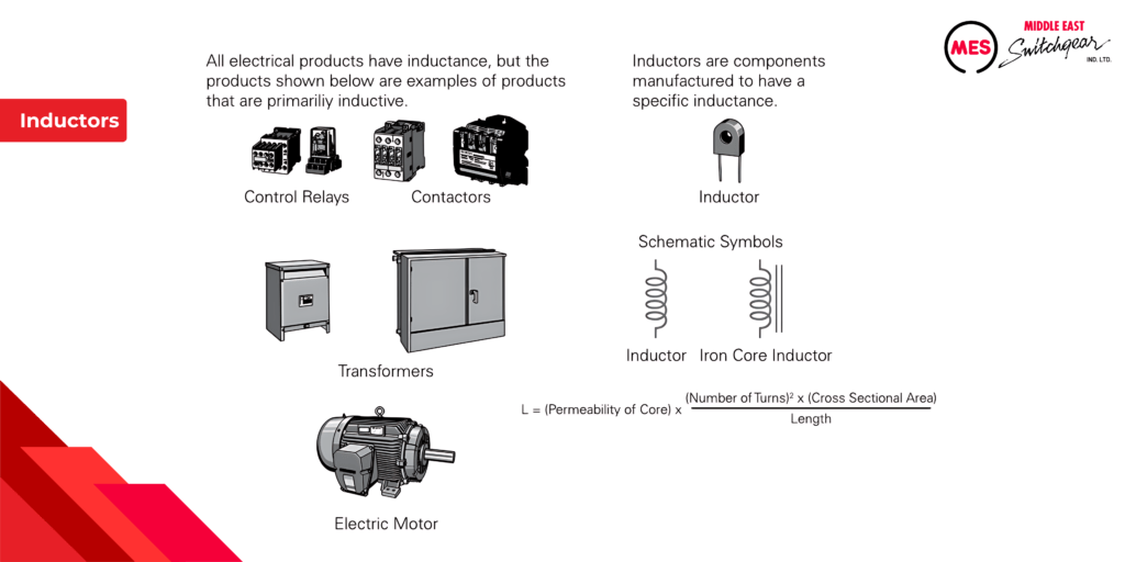
Inductors:
While all conductors have some inductance, special components called inductors are designed to maximize this effect. They’re coils of wire, sometimes wrapped around a core material, and are symbolized as curled lines in circuits.
Key Factors Affecting Inductance:
- Number of turns in the coil
- The diameter and length of the coil
- Core material (if present)
Unit
Symbol
Equivalent Measure
millihenry
mh
1 mh = 0.001 h
microhenry
µh
1 µh = 0.000001 h
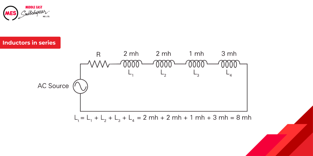
Inductors in Series
In the following circuit, an AC source supplies electrical power to four inductors.Total inductance of series inductors is equal to the sum of the inductances.
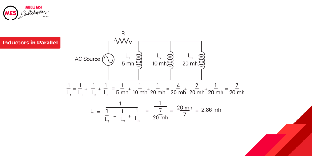
Inductors in Parallel
The total inductance of inductors in parallel is calculated using a formula similar to the formula for resistance of parallel resistors. The following illustration shows the calculation for a circuit with three parallel inductors.
Capacitance and Capacitors
Capacitance is a measure of a circuit’s ability to store an electrical charge. A device manufactured to have a specific amount of capacitance is called a capacitor. A capacitor is made up of a pair of conductive plates separated by a thin layer of insulating material. Another name for the insulating material is dielectric material. A capacitor is usually indicated symbolically on an electrical drawing by a combination of a straight line with a curved line or two straight lines.
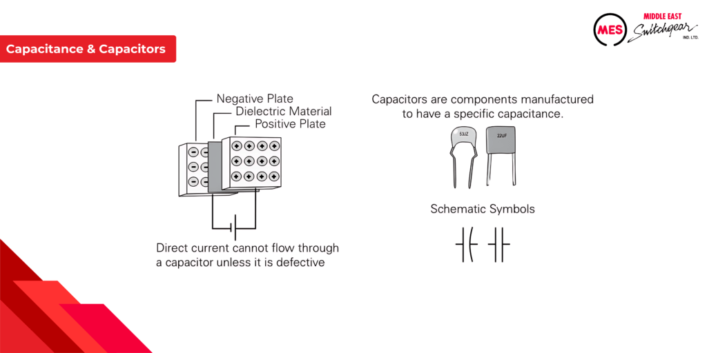
Capacitors store electrical energy. When voltage is applied, electrons accumulate on one plate and are removed from the other, creating an electric field. This doesn’t involve actual current flow through the insulating material (dielectric) separating the plates.
Capacitance:
The ability of a capacitor to store charge is called capacitance (C) and depends on:
- Plate area: Larger plates hold more charge.
- Plate separation: Closer plates increase capacitance.
- Dielectric material: Certain materials enhance capacitance.
Capacitance is measured in farads (F), but microfarads (µF) and picofarads (pF) are more common due to smaller component sizes
Unit
Symbol
Equivalent Measure
microfarad
µF
1 µF = 0.000001 F
picofarad
pF
1 pF = 0.000000000001 F
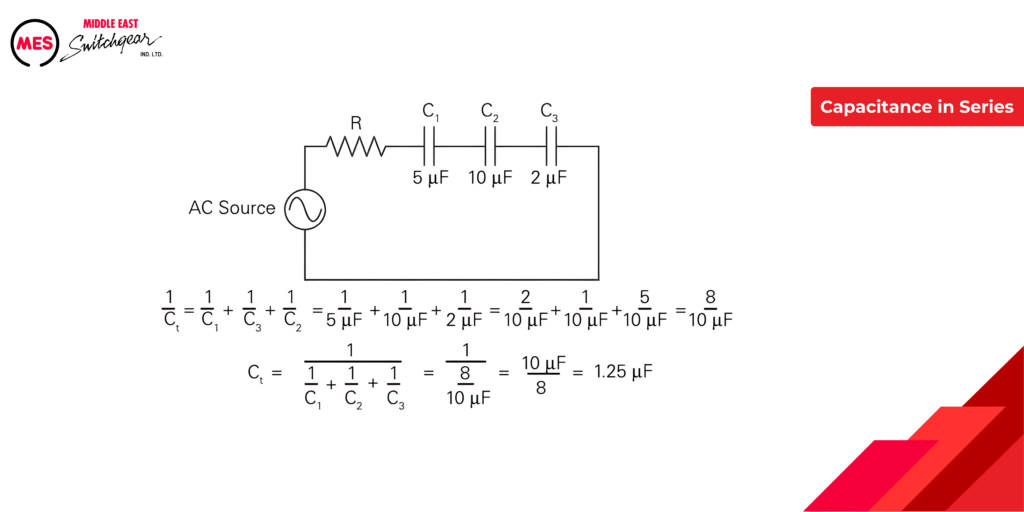
Capacitors in Series
Unlike parallel capacitors (which add capacitance), connecting capacitors in series decreases their total capacitance. This behavior is similar to how resistors behave in series.
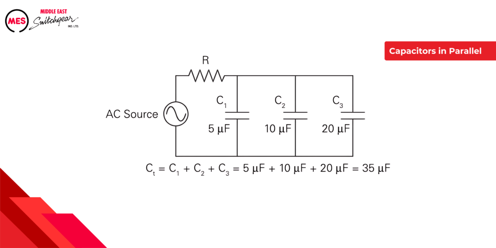
Capacitors in Parallel
Adding capacitors in parallel increases circuit capacitance. In the following circuit, an AC source supplies electrical power to three capacitors.Total capacitance is determined by adding the values of the capacitors.
Reactance and Impedance
In AC circuits, resistance isn’t the only player. Here’s what you need to know:
- Reactance (X): The opposition to current flow caused by inductors (opposing current changes) and capacitors (opposing voltage changes). Measured in ohms (Ω).
- Impedance (Z): The total opposition to current flow in an AC circuit, combining both resistance and reactance. It also acts like resistance and is measured in ohms (Ω).
Think of reactance as specific roadblocks (inductors and capacitors) affecting current flow, while impedance is the entire journey’s resistance, including those roadblocks.
Inductive Reactance
Inductive Reactance: Inductors Fight Current Changes
In AC circuits, inductors oppose changes in current flow through inductive reactance (XL). This opposition increases with both:
- Inductance value (L): Stronger inductors create more reactance.
- Frequency (f): Higher frequencies lead to greater reactance.
The formula to calculate inductive reactance is:
- XL = 2πfL= 2 x 3.14 x frequency x inductance
Example:
A 60 Hz circuit with a 10mH inductor has an inductive reactance of 3.77 ohms (calculation shown in the original passage). This reactance acts like resistance in the circuit, allowing us to use Ohm’s Law to find the current if the voltage is known.
Capacitive Reactance
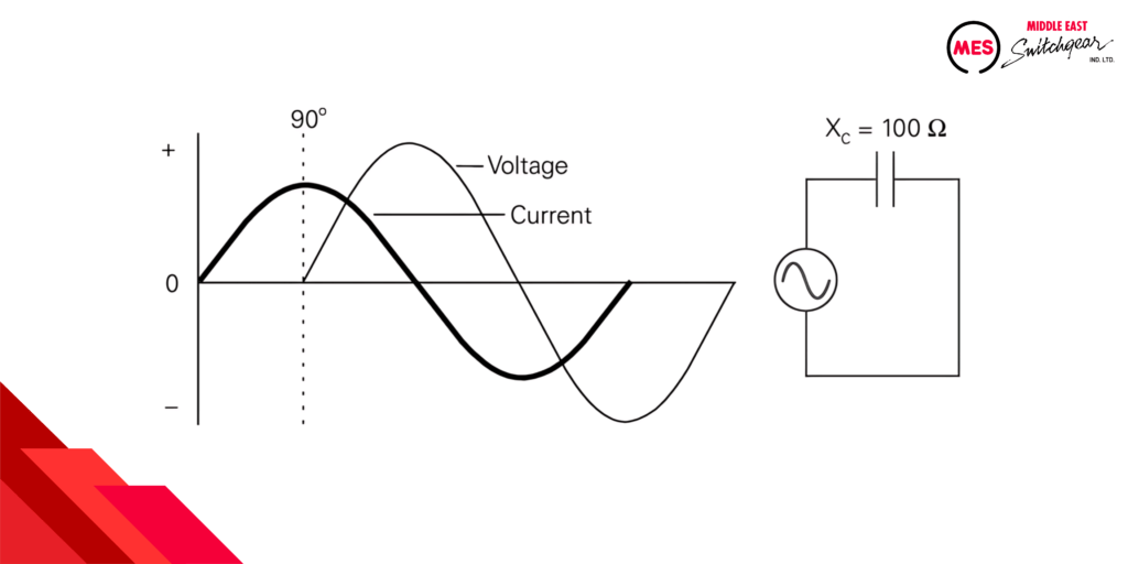
Circuits with capacitance also have reactance. Capacitive reactance is designated by the symbol XC. The larger the capacitor, the smaller the capacitive reactance. Current flow in a capacitive AC circuit is also dependent on frequency. The following formula is used to calculate capacitive reactance.
XC = 1/2πfC
The capacitive reactance for a 60 Hz circuit with a 10 mF capacitor is calculated as follows.
XC = 1/2πfC = 1/2 x 3.14 x 60 Hz x 0.000010 F = 265.39 Ω
For this example, the resistance is zero so the impedance is equal to the reactance. If the voltage is known, Ohm’s law can be used to calculate the current. For example, if the voltage is 10 V, the current is calculated as follows.
I = E/Z = 10V/265.39Ω = 0.0376 A
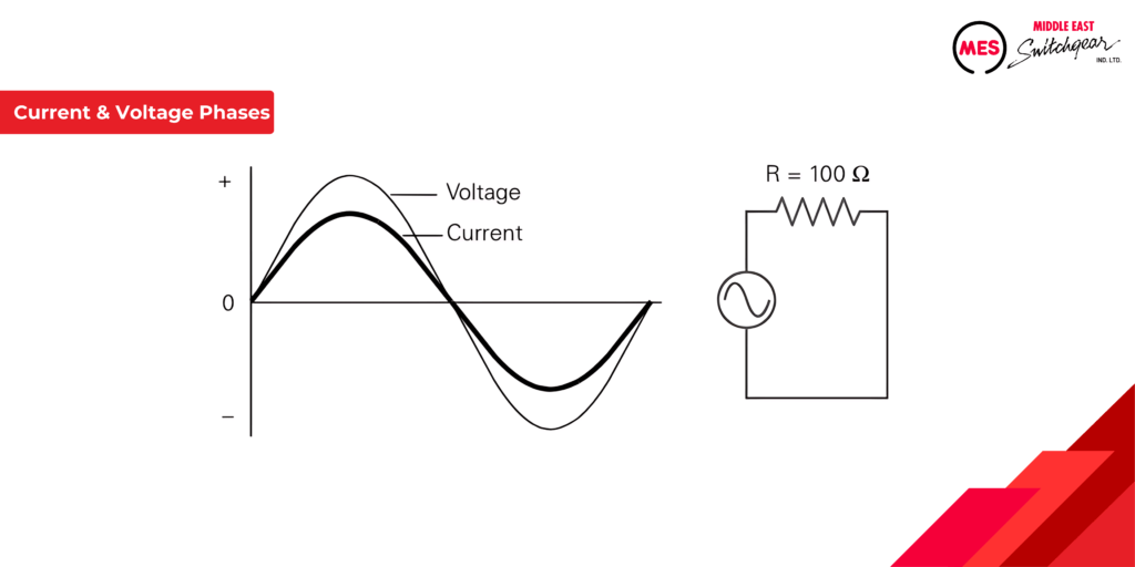
Current and Voltage Phases
In a purely resistive AC circuit, current and voltage are said to be in phase current because they rise and fall at the same time as shown in the following example.
In AC circuits with inductors, current and voltage aren’t perfectly in sync. This is called a phase shift. Here’s the key point:
- Current lags voltage by 90 degrees: The voltage “peaks” earlier than the current in the cycle.
This means the current is always “playing catch-up” to the changes in voltage due to the inductor’s opposition.
In circuits with both resistance and inductance, the phase shift between voltage and current depends on their balance:
- More Resistance (Less Reactive): Current lags voltage by less than 90 degrees, approaching being in phase (like a purely resistive circuit).
- More Inductance (More Reactive): Current lags voltage by closer to 90 degrees (like a purely inductive circuit).
The greater the influence of inductance (reactance), the more significant the lag. The example with equal resistance and inductance shows a 45-degree lag, highlighting this balancing act.
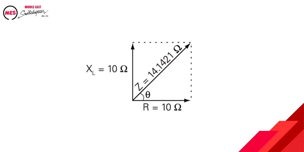
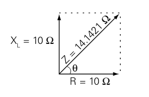
Calculating Impedance in an Inductive Circuit
When calculating impedance for a circuit with resistance and inductive reactance, the following formula is used.
Z = √R2+XL 2
For example, if resistance and inductive reactance are each 10 W, impedance is calculated as follows.
Z = √102 + 102 = √200 = 14.1421 Ω
Vector
Vectors (think arrows with direction and strength) are a powerful tool to visualize AC circuits. These diagrams show how components like resistance (R) and inductive reactance (XL) interact.
- Vector Length: Represents the magnitude (strength) of the value (e.g., voltage, current).
- Phase Angle (φ): The angle between vectors indicates how much current lags (or leads) voltage.
For example, a diagram with equal R and XL (10 ohms) would show a 45° phase angle, signifying a current lag of 45°.
Capacitive Reactance
Capacitors, alongside inductors, introduce another type of opposition to current flow in AC circuits called capacitive reactance (XC). This reactance is interesting because:
- Unlike resistance, it decreases as capacitance increases (larger capacitors oppose current less).
- It’s also frequency-dependent. Higher frequencies experience lower capacitive reactance.
The formula to calculate capacitive reactance is:
XC = 1/2πfC
The capacitive reactance for a 60 Hz circuit with a 10 mF capacitor is calculated as follows.
XC = 1/2πfC = 1/2×3.14x60Hzx0.000010F = 265.39 Ω
For this example, the resistance is zero so the impedance equals the reactance. If the voltage is known, Ohm’s law can be used to calculate the current. For example, if the voltage is 10 V, the current is calculated as follows.
I = E/Z = 10 V/265.39 Ω = 0.0376 A
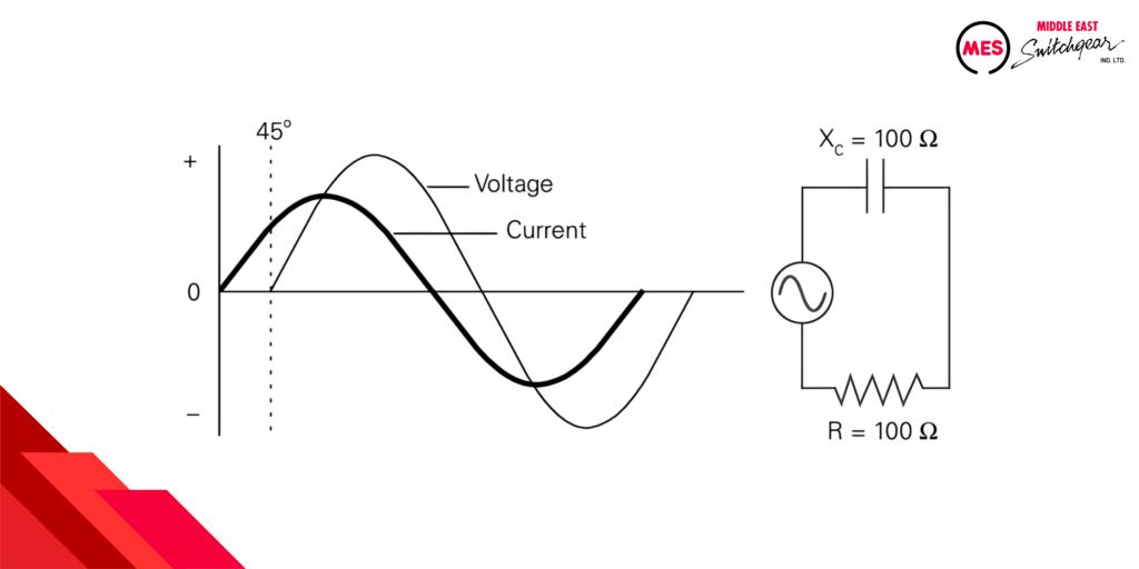
Current and Voltage Phases
Capacitive circuits exhibit a different behavior compared to inductors. Here’s the key takeaway:
- Current leads voltage by 90 degrees: The current “peaks” earlier than the voltage in the cycle.
This opposite phase shift happens because capacitors readily accept changes in voltage, causing the current to anticipate those changes.
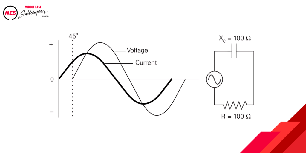
Similar to RL circuits, resistance and capacitance also influence phase shift:
- More Resistance (Less Reactive): Current leads voltage by less than 90 degrees, approaching being in phase (like a purely resistive circuit).
- More Capacitance (More Reactive): Current leads voltage by closer to 90 degrees (like a purely capacitive circuit).
The greater the influence of capacitance (reactance), the more significant the lead. The example with equal resistance and capacitance shows a 45-degree lead, highlighting this balancing act.
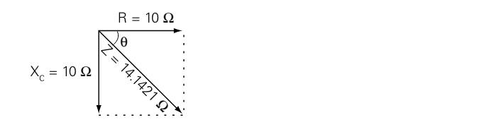
Calculating Impedance in a Capacitive Circuit
The following formula calculates impedance in the circuit with resistance and capacitive reactance.
Z = √R2 + XC2
For example, if resistance and capacitive reactance are each 10 ohms, impedance is calculated as follows.
Z = √102+102 = √200 = 14.1421 Ω
Just like inductors, capacitors introduce their own twist to AC circuits through capacitive reactance (XC). This reactance works differently:
- Opposes current, but less with larger capacitors (opposite of inductors).
- Decreases with higher frequencies.
Similar to inductive circuits, vector diagrams are a powerful tool to understand this behavior.
- Vector Length: Represents the magnitude (strength) of the value (e.g., voltage, current).
- Phase Angle (φ): The angle between vectors indicates how much current leads (opposite of inductors) voltage.
For instance, a diagram with equal resistance (R) and capacitive reactance (XC) (both 10 ohms) would show a 45° phase angle, signifying a current lead of 45°.
Remember, vector diagrams provide a clear picture of how capacitance interacts with resistance in AC circuits.
Series and Parallel R-L-C Circuits
Imagine electricity flowing through a circuit like music. In a perfect world, everything would be in sync, but reactive components like inductors and capacitors add a twist. Here’s how they affect the flow of current (electrons) relative to voltage (the electrical pressure):
- Resistance (R): The steady gatekeeper, simply opposing current flow.
- Inductance (L): The reluctant follower, causing current to lag behind voltage by 90 degrees.
- Capacitance (C): The eager forerunner, making current lead voltage by 90 degrees.
Visualizing the Dance with Vector Diagrams
Think of arrows representing voltage and current. In a perfect circuit (with just resistance), these arrows would point in the same direction. But when inductors and capacitors join the party, their influence creates a phase shift.
- Inductive Reactance (XL): Represented by a positive arrow on the imaginary axis, 180 degrees apart from capacitive reactance.
- Capacitive Reactance (XC): Represented by a negative arrow on the imaginary axis, due to its opposing effect on phase shift.
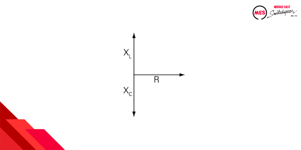
Net Reactance: Finding the Balance
In circuits with both inductors and capacitors, their reactance values (XL and XC) compete. We calculate the net reactance by subtracting XC from XL.
- Positive net reactance: Inductive influence dominates, with current lagging the voltage.
- Negative net reactance: Capacitive influence dominates, with current leading the voltage.
- Zero net reactance: The circuit behaves like a pure resistance, with current and voltage in sync.
An AC circuit is:
- Resistive if XL and XC are equal
- Inductive if XL is greater than XC
- Capacitive if XC is greater than XL
The following formula calculates the total impedance for a circuit containing resistance, capacitance, and inductance.
Z = √R2+(XL– XC )2
In the realm of AC circuits, understanding the interplay between inductive and capacitive reactance is paramount. These reactance values, denoted as XL and XC respectively, influence the phase relationship between current and voltage.
- Inductive Reactance (XL): This parameter reflects the opposition to current flow changes introduced by inductors. A higher XL signifies a greater lagging effect, causing the current to reach its peak value after the voltage peak.
- Capacitive Reactance (XC): Capacitors, on the other hand, exhibit a contrasting behavior. Capacitive reactance opposes changes in voltage itself. A higher XC leads the current to reach its peak value before the voltage peak.
Net Reactance: Determining the Dominant Influence
In a circuit containing both inductors and capacitors, the net reactance plays a crucial role. It’s calculated by subtracting the capacitive reactance (XC) from the inductive reactance (XL).
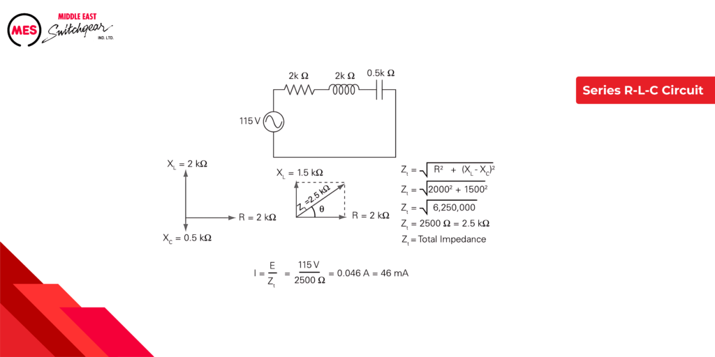
Series R-L-C Circuit
The following example shows a total impedance calculation for a series R-L-C Circuit. Once total impedance has been calculated, current is calculated using Ohm’s law.
Imagine the electrical world is a dance party, but the dance moves (reactance) change with the music’s tempo (frequency) in AC circuits!
- Inductive Reactance (The Laggard): The party pooper who resists current flow changes more as the music speeds up (frequency increases).
- Capacitive Reactance (The Eager Beaver): Gets less uptight (reactance decreases) with faster music, allowing current to flow more easily.
Series Resonance
Now, picture this: a special moment where the laggard (inductor) and the eager beaver (capacitor) cancel each other out at a specific musical tempo (frequency). This is called series resonance. Here’s what happens:
- All the reactance drama disappears, leaving only pure resistance.
- The current flows freely, like in a normal circuit (current = voltage/resistance).
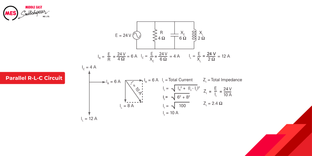
Parallel R-L-C Circuit
Unlike series circuits, parallel AC circuits with inductors and capacitors present a challenge. Inductors cause current to lag voltage, while capacitors make it lead. To analyze these circuits, we first need to determine the net reactive current by subtracting the capacitive current from the inductive current. This paves the way for calculating the circuit’s total impedance.
The total current for the circuit can be calculated as shown in
the following example. Once the total current is known, the
total impedance is calculated using Ohm’s law.
Imagine a circuit with an inductor (the resistor) and a capacitor (the free spirit) – their reactions to changing music tempos (frequency) are different!
- The Inductor (Resister): Gets stiffer (higher reactance) with faster music, making current flow less easily.
- The Capacitor (Free Spirit): Loosens up (lower reactance) with faster tempos, allowing more current to flow.
Parallel Resonance
Now, picture this: a special musical note (frequency) where the uptight resistor (inductor) and the loose free spirit (capacitor) perfectly balance each other out. This magical state is called parallel resonance. Here’s the result:
- Their opposing effects cancel out, leaving only the easy-flowing current (resistance).
- The circuit acts like a normal one, with current flowing freely (current = voltage/resistance).
Power and Power Factor in an AC Circuit
In the world of AC circuits, power isn’t as straightforward as it seems. Let’s break down the key players:
- True Power: The rate at which energy gets used (think heat from a resistor). It’s like the actual work done by the circuit.
- Reactive Power: Inductors and capacitors don’t directly consume energy, but they play a juggling act with it. They store and release energy as the current changes direction, requiring the source to generate extra “non-working” energy.
The Power Dance:
Imagine voltage and current as dance partners. When they’re in perfect sync (like in a purely resistive circuit), all the power is true power (working together). However, when they’re 90 degrees out of phase (purely capacitive or inductive), the positive and negative power peaks cancel each other out, resulting in zero average true power.
Apparent Power: The Big Picture
This combines both true and reactive power, giving us a complete picture of the total power demanded by the circuit. It’s like the overall energy required, even if not all of it gets used for actual work.
Finding the Balance: Resistance vs. Reactance
In a purely resistive circuit, true power equals apparent power because there’s no reactive juggling. Interestingly, the same happens when the inductive and capacitive reactance cancel each other out (imagine perfectly balanced dance partners). But in most real-world circuits, apparent power will be a combination of both true and reactive power.
The formula for apparent power is shown below.The unit of measure for apparent power is the volt-ampere (VA).
Power Formulas
P = EI
True power is calculated from another trigonometric function, the cosine of the phase angle (cos θ). The formula for true power is shown below. The unit of measure for true power is the watt (W).
P = EI cos θ
Imagine a circuit like a well-oiled machine. Understanding how it uses power is key! Here’s the breakdown for AC circuits:
Purely Resistive Circuit (The In-Sync Duo):
- Current and voltage are perfect partners, moving in sync (0 degrees apart).
- This perfect harmony means all the power is true power, used for work (like heat from a resistor).
- Think of it as 100% efficiency – all the energy goes towards doing the actual job.
Purely Reactive Circuit (The Out-of-Sync Dancers):
- Inductors and capacitors are like dancers out of step (90 degrees apart).
- They store and release energy as current changes direction, but don’t consume any themselves (zero true power).
- This back-and-forth creates a demand for extra energy the circuit doesn’t use, called reactive power.
- It’s like having to generate more power for the dance floor, even though the dancers aren’t using it all.
The Power Math: Cosine Connection
Engineers use the cosine function and phase angle to calculate power in AC circuits. But for a simpler understanding:
- In a purely resistive circuit (0-degree phase angle), the cosine is 1, so true power equals total power.
- In a purely reactive circuit (90-degree phase angle), the cosine is 0, resulting in zero true power consumption.
Reactive Power: The Invisible Player
While reactive power itself isn’t consumed, it’s an essential concept for efficient power delivery. By understanding it, engineers can:
- Reduce energy waste: Minimize the need for extra power generation due to reactive components.
- Improve power system efficiency: Ensure smooth energy flow and avoid overloading the system.
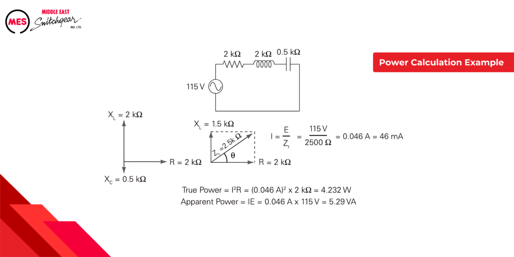
Power Calculation Example
The following example shows true power and apparent power calculations for the circuit shown.
Power Factor
Imagine a circuit like a delivery system. The goal? To get as much of the delivered power used for actual work. This is where power factor comes in:
Power Factor: The Efficiency Gauge
- It’s the ratio of true power (usable energy) to apparent power (total delivered energy).
- Think of it as a percentage score for how effectively the circuit utilizes the power it receives.
The Perfect Score: Purely Resistive Circuit
- Here, current and voltage are in perfect sync (0 degrees apart).
- Since all the power is true power (used for work), the power factor is a perfect 1.
- It’s like a perfectly efficient delivery – all the power goes towards doing the job.
Understanding Power Factor Improves Efficiency
Knowing the power factor helps engineers optimize AC circuits for better performance:
- Identify areas for improvement: A low power factor indicates wasted energy due to reactive components (inductors and capacitors).
- Reduce energy consumption: By correcting the power factor, you can minimize the need for extra power generation.
- Improve overall system health: A good power factor ensures smooth operation and prevents overloading the power system.
We saw how purely resistive circuits have a perfect power factor (1) because all the delivered power gets used. But what about reactive circuits (inductors and capacitors)?
Out-of-Sync Dance, Zero Power Factor:
- In purely reactive circuits, voltage and current are out of step by 90 degrees.
- Since the cosine of 90 degrees is zero, the power factor becomes zero.
- This doesn’t mean all the power is returned to the source (although some exchange happens). It means no true power is consumed for work.
The 80/20 Rule (Understanding Power Factor Values):
- A power factor of 0.8, for example, tells a different story.
- It indicates the circuit utilizes 80% of the delivered power for actual work (true power).
- The remaining 20% is not returned to the source but rather represents the reactive power exchange.
Power Factor: Beyond Simple Consumption
Remember, the power factor is about efficiency, not just consumption:
- A low power factor: Indicates wasted energy due to reactive components. It’s like having a delivery system where a significant portion of the delivered goods aren’t used.
- A high power factor: Means the circuit utilizes most of the received power effectively. It’s like a well-oiled delivery system with minimal waste.
Understanding power factor helps engineers design efficient AC circuits that:
- Minimize energy waste: Reduce the need for extra power generation due to reactive components.
- Improve power system health: Ensure smooth energy flow and prevent overloading the system.
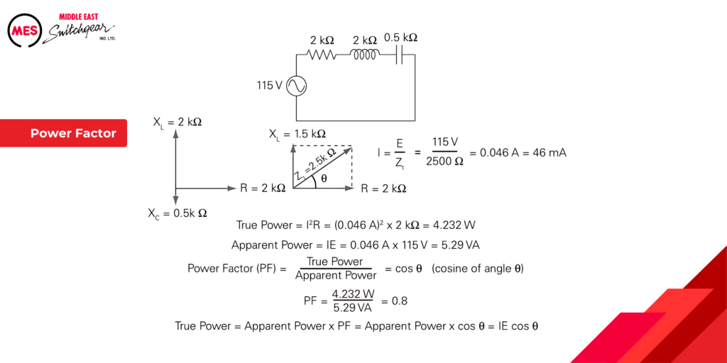
Another way of expressing true power is as the apparent power times the power factor.This is also equal to I times E times the cosine of the phase angle.
Transformers
Imagine needing to deliver water to different parts of a city. Pipes of different sizes help control the water pressure. Transformers do something similar for electricity!
What is a Transformer?
- It’s an ingenious device that transfers electrical energy from one circuit to another using a magnetic field.
- Think of it as a magic box that can change the “voltage pressure” of electricity.
Mutual Induction:
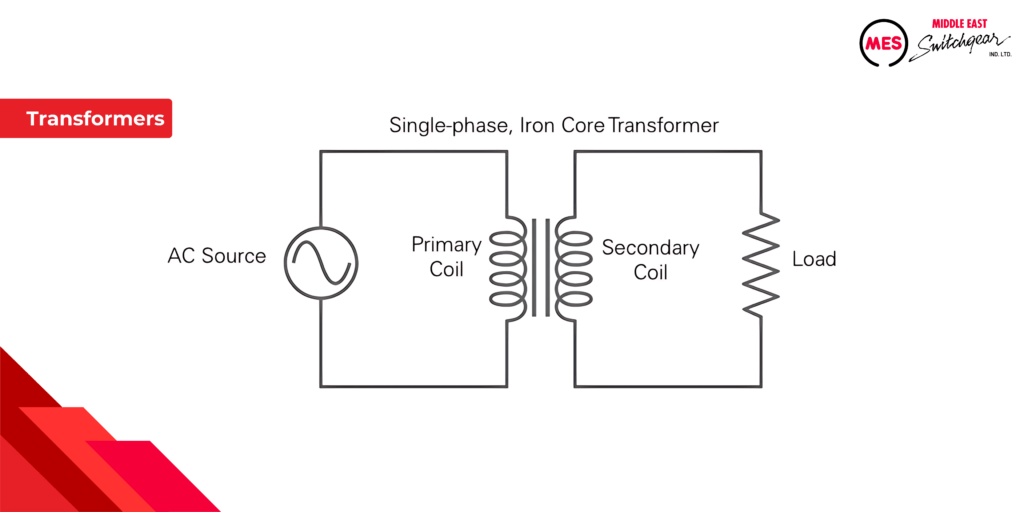
- A transformer has two coils: a primary (gets the electricity) and a secondary (sends it out).
- When electricity flows through the primary coil, it creates a magnetic field.
- This magnetic field, like an invisible handshake, transfers energy to the secondary coil, inducing a voltage in it.
Stepping Up or Stepping Down Voltage:
- Transformers can be voltage chameleons! They can:
- Step-up voltage: Increase the voltage to a higher level (like using a booster pump for water pressure).
- Step-down voltage: Decrease the voltage to a lower level (like reducing water pressure for homes).
- Transformers can be voltage chameleons! They can:
The Power of Efficiency
- Power companies generate electricity at high voltage (think high water pressure) for efficient transmission over long distances.
- Transformers at substations then step down the voltage for local distribution (like reducing pressure for neighborhoods).
- Finally, transformers near homes further step down the voltage for safe appliance use (like lowering pressure for individual houses).
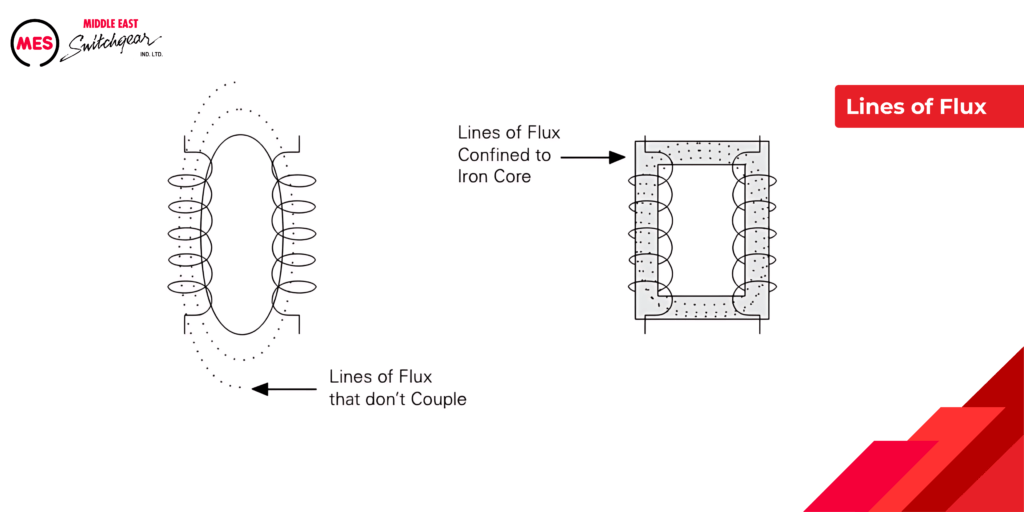
The Iron Core
- To maximize the transfer of energy, transformers use an iron core to guide the magnetic field between the coils.
- It’s like having a special pipe that ensures all the water pressure gets directed where it needs to go.
Transformers can step-up or step-down voltage. The secret lies in the number of turns in each coil:
- More Turns (Secondary) = Stepped-Up Voltage (Imagine a magnifying glass for electricity)
- Less Turns (Secondary) = Stepped-Down Voltage (Think spreading out light for even coverage)
- Equal Turns = No Voltage Change (Input equals output)
By understanding these ratios, you can predict voltage changes and choose the right transformer for your needs!
Transformer Formulas
There are several useful formulas for calculating, voltage, current, and the number of turns between the primary and secondary of a transformer. These formulas can be used with either step-up or step-down transformers. The following legend applies to the transformer formulas:
ES = secondary voltage
EP = primary voltage
IS = secondary current
IP = primary current
NS = turns in the secondary coil
NP = turns in the primary coil
To find voltage:
ES = EP x IP/IS
EP = ES x IS/IP
For example, suppose a transformer has a primary voltage of 240 V, a primary current of 5 A, and a secondary current of 10 A. In that case, the secondary voltage can be calculated as shown below.
ES = EP x IP/IS = 240Vx5A/10A = 1200/10 = 120V
To find current:
IS = EP x IP/ES
IP = ES x IS ES/EP
To find the number of coil turns:
NS = ES x NP/EP
NP = EP x NS/ES
Transformer Ratings
Transformers are rated for their apparent power capacity in kVA (kilovolt-amperes). This rating is crucial to avoid overheating. For single-phase transformers, multiply the secondary voltage by the maximum load current to get the kVA rating.
Example:
A transformer needs to provide 240V at 75A. Minimum kVA rating: 240V x 75A = 18 kVA
Transformer Losses
While transformers efficiently transfer most power, some energy is lost:
- Heat Loss: A small amount of energy heats the wires and core.
- Core Losses Reduced by Laminations: Building the transformer core from thin, layered sections (laminations) helps minimize these losses.
Even small efficiency improvements make a big difference in large-scale power systems!
Three-Phase AC
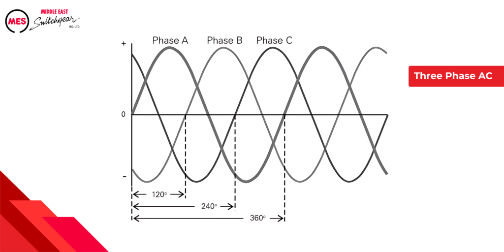
Our homes and offices typically use single-phase power, delivered as a single AC wave.
For higher power needs, like in factories, industries, and power grids, three-phase power takes center stage. It’s like having three synchronized AC waves delivering power simultaneously, each offset by 120 degrees, for a more efficient and powerful delivery system.
Three-Phase Transformers
Three-phase transformers are used when power is required for larger loads such as industrial motors. There are two basic three-phase transformer connections, delta and wye.
Delta Connections
In the world of three-phase power, a critical player emerges: the delta transformer. These transformers are like the workhorses of industrial and commercial power distribution, visualized as triangles in schematics.
Why Triangles? Decoding the Phases:
Each side of the triangle represents a single phase (voltage) within the three-phase system. Imagine three lanes carrying electrical energy simultaneously – that’s the essence of three-phase power!
Key Advantage: Consistent Voltage Delivery
Here’s a crucial benefit of delta transformers: the voltage measured between any two terminals of the delta remains constant. No matter which two “lanes” you connect (e.g., L1 and L2), you get the same voltage.
Powering Diverse Needs: Single-Phase and Three-Phase Applications
The versatility of delta transformers shines through when it comes to supplying power:
- Single-Phase Needs: For regular appliances requiring only one phase, a single voltage can be conveniently extracted from the delta configuration (like L1 to L2).
- Three-Phase Powerhouses: When it comes to high-power equipment in factories and industries, all three phases can be harnessed simultaneously. The delta transformer acts as a conductor, delivering the combined power of all three phases.
Remember: Just like single-phase transformers, the delta transformer’s output voltage depends on two key factors:
- Incoming Voltage (Primary): The voltage level entering the transformer.
- Turns Ratio: The ratio between the number of turns in the primary and secondary coils. This ratio dictates the voltage transformation achieved by the transformer.
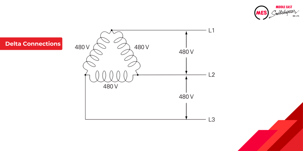
When current is the same in all three coils, it is said to be balanced. In each phase, current has two paths to follow. For example, current flowing from L1 to the connection point at the top of the delta can flow down through one coil to L2, and down through another coil to L3. When current is balanced, the current in each line is equal to the square root of 3 times the current in each coil.
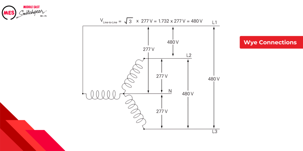
Wye Connection
Wye transformers (also called star transformers) are another key player in three-phase power systems. They’re depicted with coils connected in a “Y” shape, offering four output leads:
- Three-phase leads: Deliver power for three-phase applications.
- One neutral lead: Provides a reference point for grounding and single-phase loads.
Understanding Line-to-Line vs. Line-to-Neutral Voltage
An important concept in wye transformers is the difference between line-to-line and line-to-neutral voltage:
- Line-to-neutral voltage: This is the voltage measured between any phase lead and the neutral lead (e.g., 277 volts in the example).
- Line-to-line voltage: This is the voltage measured between any two phase leads (e.g., 480 volts in the example). Here’s the key formula: Line-to-Line Voltage = √3 (Line-to-Neutral Voltage)
Wye Transformers: A Versatile Choice
The presence of a neutral lead makes Wye transformers well-suited for applications requiring both single-phase and three-phase power.